The Hitchhiker’s Guide to Training on Compute Islands
We think learning algorithms for the frontier should be codeveloped to maximally utilize the compute in this world.
tl;dr: A position on training across clusters, and a call to action on truly distributed learning. We trained a sparse mixture-of-experts model across two clusters of different sizes, with different types of GPUs, nearly halfway around the world from each other, over a bidirectional link of 25 Gbps. It was glorious. We also revisited butterfly mixing, replacing the all-reduce with pairwise exchanges between eight learners, and it matched standard training.
Training compute rarely arrives as one big contiguous block. The market has far more availability in scattered clusters, from a few hundred to a few thousand GPUs, spread across many neoclouds. Added together, these resources can be substantial.
The biggest bottleneck in deployment of accelerated compute is not the chips themselves but power, grid equipment and land, and prediction is that they will stay that way until 2028. Microsoft CEO Satya Nadella said plainly in words “you may actually have a bunch of chips sitting in inventory that I can’t plug in” (DCD).
Developers and utilities remain misaligned on time-to-power, with gaps widening in key hubs (Bloom Energy). Gas turbines are spoken for through 2028 (Bloomberg), and large transformers now take more than three years to arrive (Reuters). Local opposition killed at least 20 projects in a single quarter (Heatmap). Goldman Sachs expects only 50–60% of the US data center capacity scheduled for the next one to two years to come online on time, down from a historical rate of about 72% (Goldman Sachs).
A site under 20 MW often plugs into the grid that’s already there, but for much larger installations, we would need substantial investments in the grid, transmission, and power plants.
Modern frontier training stacks assume a single colocated cluster due to the predominant use of well-understood synchronous distributed training. In this work, we explore less popular, but emerging works from the past decade in distributed training. As we see it, the bottleneck that holds most organizations back is not the raw amount of compute, but the ability to turn islands of compute into one valuable frontier training run.
Stranded, or just inconvenient?
On October 25, Elon Musk put the problem bluntly:
“I think we’re going to see a lot of stranded compute in partially complete data centers.”
Elon Musk on X, October 25, 2026Open on X ↗
In the same exchange on X, someone pointed out that demand for accelerators to build and serve intelligence is still insatiable. Musk replied that this only helps if you can get the compute online and running reliably, which he called “extremely difficult to do at scale” (X).
So the problem is not only a lack of power at the campus. It is the wider gap between owning GPUs and reliably turning them into valuable tokens, including putting them to work in a frontier training run.
If a team’s training stack could use compute wherever it is, in whatever sizes and for however long it becomes available, how much more frontier training compute would that team actually have?
There are two problems here:
The physical problem
Hardware in an unfinished building needs power, cooling, networking and money.
The architectural problem
A perfectly healthy cluster can still be useless for a job that expects one large, uniform cluster that never goes down.
Software can do nothing about the first problem. The second is squarely within its reach.
Our case rests on a growing literature and increasingly capable training runs. Our contribution in this blog is a practical case study in two parts. First, a mixture-of-experts model with roughly 32B total parameters, 32x sparsity was trained across two clusters about 9,000 miles apart. Notably, these clusters had different accelerators (GB300 and B300), different parallelism schemes and different total batch sizes. This could allow us to mix in more accelerator types to get to a particular compute budget. Second, we replaced the all-reduce with butterfly mixing, where learners exchange model fragments in pairs.
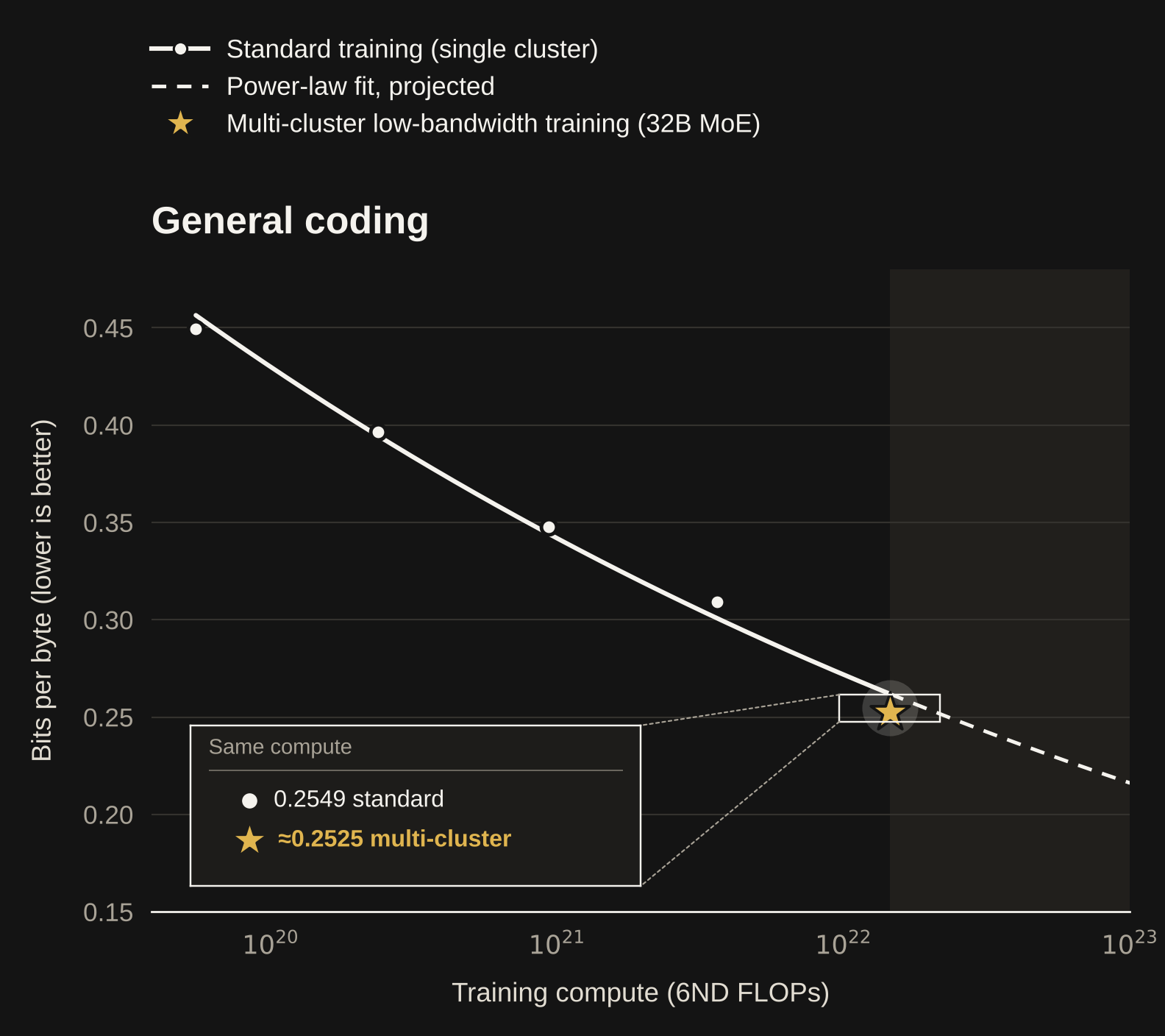
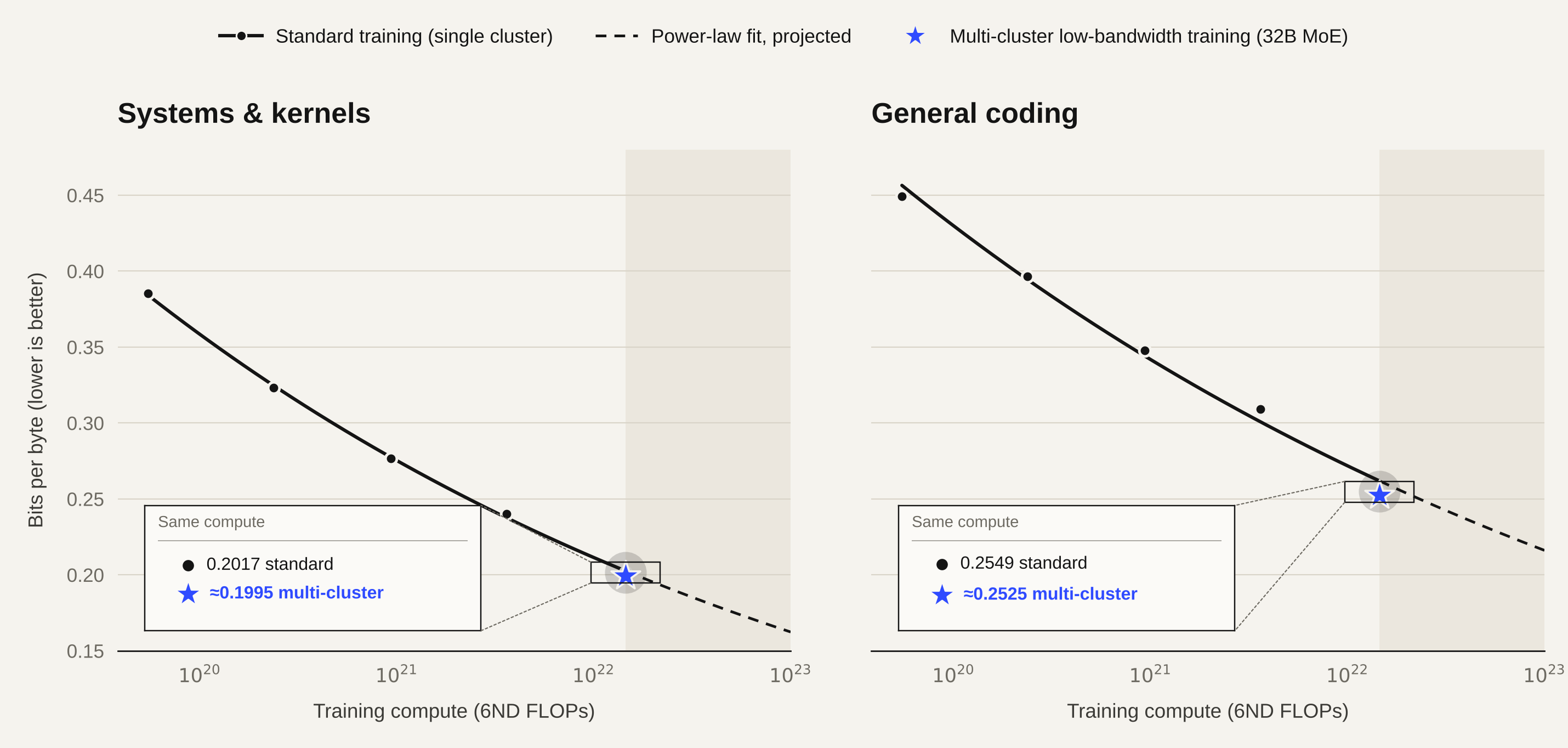
We combined better transport scheduling, error feedback on communication, robust failure handling and a stronger optimization method derived from Distributed Shampoo, building on existing work such as DiLoCo. At the same compute, training across the two sites reached about 1% lower bits per byte than standard training on both of our evals.
Compute comes in many shapes
The market already sells compute in very different shapes, from multiyear contracts down to a single node for an hour.1
Committed
Large, predictable allocations on multiyear terms.
Nebius and CoreWeave sold multiyear capacity to Microsoft and Meta, in deals worth up to $19.4 billion.
Reservable
Clusters of tens to hundreds of GPUs.
AWS, Lambda and Together AI rent clusters from a single node to hundreds of GPUs, for hours to months.
Spot & resale
Short-term and unused capacity.
SF Compute sells GPU time by the hour and lets buyers resell what they don’t use; the National Compute Grid pools idle capacity across clouds.
A brief history of low-communication training
Low-communication training is older than the current LLM scaling cycle. The idea of synchronizing parallel workers less often goes back decades and keeps being rediscovered, most visibly in federated learning. There are four lines of work, most of them from the 2010s, which underpin today’s methods:
- Local updates. Local SGD and federated averaging take many steps between exchanges.
- Compression. Quantization, sparsification and low-rank methods shrink the bytes sent and received in each exchange.
- Gossip. Each node talks to only a subset of peers.
- Fault-tolerant averaging. Methods such as Downpour SGD cope with unreliable peers.
Federated learning added two more ingredients: treat each worker’s parameter change between exchanges as a pseudo-gradient, and apply a separate outer optimizer to it. Since 2022 these ideas have been tested on large language models, with good evidence about optimization quality, elasticity and cost.
It is also worth noting there are two different families here, as they address different constraints, and can be combined together.
Foundations, before 2022
| Year | Work | Contribution |
|---|---|---|
| 2010 | Parallelized SGD (Zinkevich et al.) | Averaging models trained independently on separate data |
| 2012 | Downpour SGD (Dean et al.) | The classic asynchronous design: training continues when individual machines are slow or fail |
| 2014 | 1-bit SGD (Seide et al., Interspeech) | 1-bit gradient quantization with error feedback |
| 2015 | Elastic Averaging SGD (Zhang et al.) | Workers are loosely tied to a central copy, so they tolerate delay and drift |
| 2016 | Federated averaging (McMahan et al.) | Many local steps on each client between averaging rounds |
| 2016 | QSGD (Alistarh et al.) | Gradient quantization with convergence guarantees |
| 2017 | D-PSGD (Lian et al.) | Decentralized SGD: nodes average with neighbors (gossip) instead of a global all-reduce |
| 2017 | Deep Gradient Compression (Lin et al.) | Sends only a small fraction of gradient values, with momentum correction |
| 2018 | Local SGD (Stich); Lin et al. | Convergence analysis and the empirical case for infrequent averaging |
| 2019 | PowerSGD (Vogels et al.) | Low-rank compression compatible with all-reduce |
| 2019 | SlowMo (Wang et al.) | Momentum applied to periodic averages; a precursor of DiLoCo’s outer optimizer |
| 2019–20 | FedAvgM (Hsu et al.); FedOpt (Reddi et al.) | Inner/outer optimizer formulation with server-side momentum and adaptive outer steps |
| 2020 | Learning@home (Ryabinin & Gusev) | Decentralized mixture-of-experts training on volunteer hardware |
| 2021 | Moshpit SGD (Ryabinin et al.) | Dynamic averaging groups for unreliable, heterogeneous peers |
| 2021 | DeDLOC (Diskin et al.) | Collaborative pretraining with volunteers, demonstrated on a Bengali ALBERT model |
Large-model era, 2022–2026
| Date | Work | Type | What the evidence adds |
|---|---|---|---|
| Jan 2023 | SWARM Parallelism | Method, model-parallel | Pipeline training on preemptible, heterogeneous devices: a transformer with 1B shared parameters on T4 GPUs over slow links. |
| Nov 2023 | DiLoCo | Method | AdamW inner optimizer, Nesterov outer optimizer, hundreds of local steps between exchanges, models up to 400M. With 8 workers it matched fully synchronous training while communicating 500× less. |
| Jul 2024 | OpenDiLoCo | Method + demo | Open implementation, models up to 1.1B, and a real run across three countries on two continents. |
| Aug–Nov 2024 | DisTrO / DeMo | Method | A separate line that compresses optimizer momentum in a transformed representation, with its own state and aggregation rules. |
| Nov 2024 | Photon | Method + system | Federated pretraining up to 7B, examining local optimization and communication trade-offs. |
| Dec 2024 | INTELLECT-1 | Run | 10B model pretrained on 1T tokens across five countries and three continents, with up to 112 H100s active at once. |
| Jan 2025 | Streaming DiLoCo | Method | Synchronizes parameter fragments in sequence, overlaps communication with computation and quantizes exchanges. Similar quality with about two orders of magnitude less bandwidth. |
| Mar 2025 | DiLoCo scaling laws | Method study | Controlled study of how model size, replica count and hyperparameters affect quality. |
| Jun 2025 | DiLoCoX | Systems experiment | Modified Qwen1.5-107B on 160 A800s over an emulated 1 Gbit/s link, 4,000 steps on WikiText-103. Useful at large parameter count, with a measurable quality gap. |
| Aug 2025 rev. 2026 |
SparseLoCo | Method | Top-k sparsification, error feedback and low-bit quantization of pseudo-gradients. |
| Jan 2026 | Pluralis Node0 | Run, model-parallel | 7.5B model trained on 36B tokens over three weeks by 303 active participants; each device held one block of the model. |
| Mar 2026 | Covenant-72B | Run | 72B model pretrained on about 1.1T tokens with permissionless participation and SparseLoCo. |
| Apr 2026 | Decoupled DiLoCo | Method + systems | Asynchronous learners, quorum-based aggregation and heterogeneous hardware. Matches data-parallel quality up to 9B under simulated failures; a real 12B run spread eight learners across four US regions (blog). |
| Jun 2026 | Factored Gossip DiLoCo | Method | Replaces part of DiLoCo’s global averaging with pairwise gossip to reduce blocking communication. |
| Jul 2026 | Agora / Pluralis-8B | Run, model-parallel | 8.6B model pretrained on 500B tokens over 40 days by 330 contributor nodes, mostly consumer GPUs. |
| Oct 2026 | Cross-facility HPC pretraining | Systems demo | A 0.6B model trained across three supercomputers on two continents, with an explicitly reported quality cost: perplexity 34.7 versus 28.2 for the centralized baseline. |
Our case study: two clusters, one model
Early on, we set ourselves a concrete challenge: could our training stack turn two separate allocations into one useful training system? We used 160 B300 GPUs in the US and 160 GB300 GPUs in Asia, roughly 9,000 miles apart.
The model was a conventional sparse mixture-of-experts (MoE) with about 32B total parameters and an MoE layer in every transformer block: 256 experts, top-8 routing and no shared experts.
We made many improvements. A few notable ones:
- Synchronization. Rather than syncing the whole model at once, we synced it fragment by fragment, staggered across each 50-step window. We borrowed fragment-wise, overlapped and asynchronous updates from Streaming and Decoupled DiLoCo. Sites exchanged updates on a 50-step schedule, and a late-arriving update can still be committed.
- Local optimizer. Each site used a variant of Distributed Shampoo.
- Communication. Exchanged values were compressed with stochastic rounding plus error feedback.
- MoE routing. The small routing statistics were coordinated and synchronized separately, at every step.
Engineering for tail latency
We rewrote the networking layer to focus on completion time of each update, and make it predictable. Thus, we optimized directly for tail latency, which involved implementing several strategies. Each of them was a simple idea, but the gains came from putting them together.
Spread demand over time
We staggered parameter updates over time, paced total traffic and capped per-socket send rates, so workers that finished together didn’t burst together. Control messages for coordination and repair ran independently, so they were never blocked.
Keep connections warm and verified
We reused warm connections, watched them with heartbeats and reconnected with jitter. We also preallocated most of the memory the transfers needed.
Chunk everything
Payloads were split into independently scheduled chunks that any healthy connection could claim as soon as it was free, so slow links couldn’t hold an update back.
Repair only what’s missing
When a write stalled, we re-requested only the missing pieces and allowed a bounded number of duplicate sends. We also launched redundant transfers when a deadline hit, which cut tail latency.
At the same compute, the two-site run reached ≈0.2525 bits per byte vs 0.2549 for standard training. Next we asked whether pairwise exchanges could replace the all-reduce.
Revisiting butterfly mixing
To find out, we split 64 GB300 GPUs at one site into eight independent cells, each an eight-GPU learner training its own copy of the 32B-parameter MoE. Instead of averaging updates across all eight cells at once, cells exchanged model fragments in pairs and kept training in between. After three rounds, every cell’s update has reached all eight, with no all-reduce. The approach dates back to Zhao and Canny’s butterfly mixing. Training quality matched the baseline.
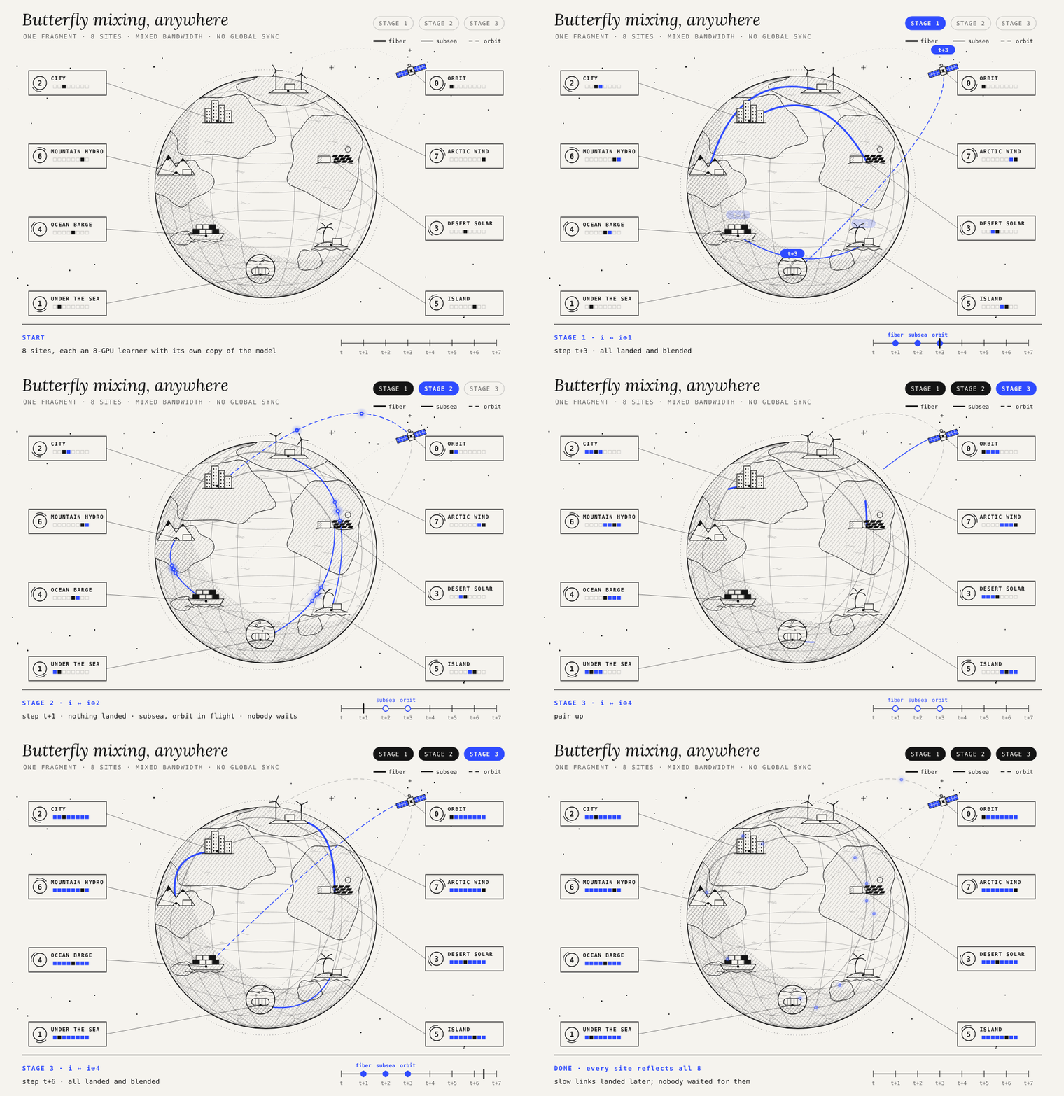
In practice, pairings differed by fragment, and each exchange was asynchronous from the cell’s point of view:
# pairings differ per fragment
fragment A:  0–5  1–3  2–6  4–7
fragment B:  0–1  2–4  3–5  6–7

# one exchange, from one cell's view
step t     build candidate from fragment, send to partner
step t+1   keep training
step t+2   live ← 0.5·live + 0.5·pair_result
The model’s parameters were divided into fragments, and each fragment was exchanged six times every 50 steps (two full butterflies), or about once every eight steps. At each exchange, a cell built a fresh outer-update candidate from its local optimizer state, sent it to its partner and kept training. Two steps later, it blended the pair’s result into its training weights at equal weight.
Varying the pairing for each fragment also spread traffic across peers and over time: each cell traded different parts of the model with different partners at the same time.
Training in orbit
The boldest version of this idea is already being tried. Google announced Project Suncatcher in November 2025, a research program exploring constellations of solar-powered TPU satellites linked by optical connections (system design). On October 30, 2026, a month after its first prototype launched, Google reported the first AI response from a data-center-class TPU in orbit: a haiku from an onboard Gemma 4 model.
That is inference on a single satellite. Training across many is a harder problem. Orbit is the extreme version of a compute island: links to the ground come and go, heat can only be radiated away, and radiation makes hardware fail more often. Those are the same problems our approach is meant to handle: learn locally through interruptions, and combine progress when a connection returns.
An ambitious first step would be to pretrain a small model across a few satellites and compare it with a ground baseline. A trillion-parameter orbital run is much further off. Science fiction has long imagined the von Neumann probe, a spacecraft that copies itself and spreads across the galaxy; ours is a humbler idea, a model that keeps learning across machines that are far apart and only sometimes connected. So we aim for the stars: if training works in orbit, it should work on any cluster on the ground.
What this means for the industry
As training reliably spans multiple smaller clusters, much more of the world’s compute becomes usable for frontier training, capacity that would otherwise go to less valuable computation. Training runs can move fungibly across clusters, surviving outages and delays that hit one region. A frontier run could even live on low-priority, preemptible capacity, taking compute when it frees up and giving it back without losing progress, which makes it fault tolerant by design. And more research teams can attempt ambitious work and scale up without first securing a gigawatt campus.
Today, the main barrier to frontier-scale training is assembling a single colocated GPU cluster, which only a few organizations can do. The lines of work we explore here widen the set of actors who can train highly capable models.
Approaches in this direction can widen the usable training pool for frontier training. Each island only runs on its own schedule, so a single run can mix accelerator generations and vendors, with different memory sizes, interconnects and parallelism layouts, as our own run already mixed GB300 and B300 clusters. Older generations or less common chips could also participate in a frontier run.
It’s also possible that integrity and safety get harder too when models are trained across providers: one faulty or compromised site can quietly degrade or tamper with the model, in ways that are harder to trace.
If you have compute islands and want to make them useful for frontier training runs, or you’re someone who wants to work with a crew pushing the boundaries of learning methods, write to hello@coreauto.com. We’re hiring across research, systems and lab automation.
Notes
- Sources for the compute tiers: CoreWeave Q3 2025 results; Nebius–Microsoft agreement (Bloomberg on the $17.4 billion and $19.4 billion figures); Nebius Q3 2025 results (Meta); Lambda 1-Click Clusters; Together AI Instant Clusters; AWS Capacity Blocks; SF Compute; National Compute Grid (HPCwire). ↩
BibTeX
@article{anil2026computeislands,
  author  = {Rohan Anil},
  title   = {The Hitchhiker's Guide to Training on Compute Islands},
  journal = {Core Automation Blog},
  year    = {2026},
  month   = {November}
}